ESTUDIOS OBSERVACIONALES: El problema de los factores de confusión.

\[OR=\frac{\Pr\left(\textrm{HTA}\left|DM\right.\right)\left/\Pr\left(\textrm{HTA}^{c}\left|DM\right.\right)\right.}{\Pr\left(\textrm{HTA}\left|{DM}^{c}\right.\right)\left/\Pr\left(\textrm{HTA}^{c}\left|{DM}^{c}\right.\right)\right.}=\frac{1.8409}{0.364}\cong5.058\]

ESTUDIOS OBSERVACIONALES: El problema de los factores de confusión.

¿Es la diabetes causa de la hipertensión arterial?

ESTUDIOS OBSERVACIONALES: El problema de los factores de confusión.

¿Es la diabetes causa de la hipertensión arterial?

¿o hay un efecto confusor de la resistencia a la insulina?

¿Cuál es aquí el papel de la edad?

Distribución de probabilidad binomial

• Consideremos un experimento aleatorio en el cuál solo son posibles dos resultados excluyentes; por ejemplo, seleccionar al azar a una persona de una población y determinar si esa persona tiene o no cierta enfermedad .

• Sea \(\pi\) la probabilidad de ocurrencia de cierto suceso de interés; por ejemplo, que la persona tenga la enfermedad .

• Supongamos que el experimento se repite \(n\) veces en las mismas condiciones, de tal forma que los sucesivos resultados sean independientes; por ejemplo, se evalúan \(n\) personas elegidas al azar en la misma población .

• Sea \(X\) = “número de ocurrencias del suceso de interés”; por ejemplo, el número de personas enfermas entre las \(n\) .

• \(X\) es, por definición, una variable aleatoria con distribución de probabilidad binomial de parámetros \(n\) y \(\pi\).

Distribución de probabilidad binomial

• Para denotar las variables aleatorias binomiales de parámetros \(n\) y \(\pi\) utilizaremos la notación: \[ X\cong b\left(n,\pi\right) \]

• Puede demostrarse que:

  • \(E\left[X\right]=n\pi\)

  • \(var\left(X\right)=n\pi\left(1-\pi\right)\)

  • \(sd\left(X\right)=\sqrt{n\pi\left(1-\pi\right)}\)

• Y también que: \[P\left(X=k\right)=\binom{n}{k}\pi^{k}\left(1-\pi\right)^{n-k}\]

Distribución de probabilidad binomial

Ejemplo

• La prevalencia estimada de HTA en la población adulta de Telde es del 31.5% (324 casos en una muestra de 1030 personas).

• Si se elige una muestra de tamaño \(n\) de esta población y se define la variable aleatoria:

  \(X\) = “Número de personas con HTA”

• Entonces \(X\cong b\left(n,0.315\right)\).

• Sabemos que la HTA se asocia con DM. Esta asociación se traduce en que el parámetro de la distribución binomial cambia según que los sujetos tengan DM o no.

Regresión logística.

La variable DM determina dos cohortes: cohorte 1 \(\cong\) {DM=Sí} y cohorte 0 \(\cong\) {DM=No}  

Si se eligiera una muestra aleatoria de tamaño \(n_i\) en la cohorte \(i\), el número de personas con HTA en esa muestra sería una variable aleatoria binomial de parámetros \(n_i\) y \(\pi\left(i\right)\), \(i=0,1\). Concretamente:

• En la cohorte 1 (personas con DM): \(X\cong b\left(n,\pi\left(1\right)=0.6482\right)\).

• En la cohorte 0 (personas sin DM): \(X\cong b\left(n,\pi\left(0\right)=0.2672\right)\).

Regresión logística.

• Si consideramos la variable

  \[I_{DM}=\begin{cases} 0 & DM=No\\ 1 & DM=Sí \end{cases}\]

• El modelo de regresión logística asume que la función \(\pi\left(i\right)\) es de la forma:

  \[\pi\left(I_{DM}\right)=Pr\left(HTA\left|I_{DM}\right.\right)=\frac{\exp\left(\beta_{0}+\beta_{1}\cdot I_{DM}\right)}{1+\exp\left(\beta_{0}+\beta_{1}\cdot I_{DM}\right)}\]

• En este caso se obtienen: \(\beta_0\) = -1.00896, \(\beta_1\) = 1.62114

• De forma que:

  • \(\pi\left(I_{DM}=1\right)=\frac{\exp\left(-1.00896+1.62114 \right)}{1+\exp\left(-1.00896+1.62114\right)} \approx 0.6484\)

  • \(\pi\left(I_{DM}=0\right)=\frac{\exp\left(-1.00896 \right)}{1+\exp\left(-1.00896\right)} \approx 0.2672\)

Estimación de la regresión logística con R

logist <- glm(HTA_OMS~DM,data=telde0,family=binomial)
summary(logist)

## 
## Call:
## glm(formula = HTA_OMS ~ DM, family = binomial, data = telde0)
## 
## Deviance Residuals: 
##     Min       1Q   Median       3Q      Max  
## -1.4459  -0.7885  -0.7885   0.9308   1.6247  
## 
## Coefficients:
##             Estimate Std. Error z value Pr(>|z|)    
## (Intercept) -1.00896    0.07525 -13.408  < 2e-16 ***
## DMSí         1.62114    0.19983   8.113 4.96e-16 ***
## ---
## Signif. codes:  0 '***' 0.001 '**' 0.01 '*' 0.05 '.' 0.1 ' ' 1
## 
## (Dispersion parameter for binomial family taken to be 1)
## 
##     Null deviance: 1282.8  on 1029  degrees of freedom
## Residual deviance: 1213.1  on 1028  degrees of freedom
## AIC: 1217.1
## 
## Number of Fisher Scoring iterations: 4

Interpretación de los coeficientes de la regresión logística

• A partir del modelo \[Pr\left(HTA\left|I_{DM}\right.\right)=\frac{\exp\left(\beta_{0}+\beta_{1}\cdot I_{DM}\right)}{1+\exp\left(\beta_{0}+\beta_{1}\cdot I_{DM}\right)}\]

• puede probarse sin mucha dificultad (ver página siguiente) que: \[OR=\frac{\Pr\left(HTA\left|DM\right.\right)\left/\Pr\left(HTA^{c}\left|DM\right.\right)\right.}{\Pr\left(HTA\left|DM^{c}\right.\right)\left/\Pr\left(HTA^{c}\left|DM^{c}\right.\right)\right.}=\exp\left(\beta_{1}\right)=e^{\beta_{1}}\]

• En este caso: \[e^{\beta_{1}} = e^{1.62114} = 5.0589\]

Demostración de que \(OR=e^{\beta_1}\)

\[OR=\frac{\Pr\left(HTA\left|DM\right.\right)\left/\Pr\left(HTA^{c}\left|DM\right.\right)\right.}{\Pr\left(HTA\left|DM^{c}\right.\right)\left/\Pr\left(HTA^{c}\left|DM^{c}\right.\right)\right.}=\]

\[=\frac{\Pr\left(HTA\left|I_{DM}=1\right.\right)\left/\Pr\left(HTA^{c}\left|I_{DM}=1\right.\right)\right.}{\Pr\left(HTA\left|I_{DM}=0\right.\right)\left/\Pr\left(HTA^{c}\left|I_{DM}=0\right.\right)\right.}=\]

\[=\frac{\frac{\exp\left(\beta_{0}+\beta_{1}\right)}{1+\exp\left(\beta_{0}+\beta_{1}\right)}\left/\left(1-\frac{\exp\left(\beta_{0}+\beta_{1}\right)}{1+\exp\left(\beta_{0}+\beta_{1}\right)}\right)\right.}{\frac{\exp\left(\beta_{0}\right)}{1+\exp\left(\beta_{0}\right)}\left/\left(1-\frac{\exp\left(\beta_{0}\right)}{1+\exp\left(\beta_{0}\right)}\right)\right.}=\frac{\exp\left(\beta_{0}+\beta_{1}\right)}{\exp\left(\beta_{0}\right)}=\exp\left(\beta_{1}\right)\]  

(hemos tenido en cuenta que \(\Pr\left(HTA^{c}\left|I_{DM}\right.\right)=1-\Pr\left(HTA\left|I_{DM}\right.\right)\))

Regresión logística: OR e intervalo de confianza con R

OR:

exp(coef(logist))

## (Intercept)        DMSí 
##   0.3645991   5.0588290

Intervalos de confianza:

exp(confint(logist))

##                 2.5 %   97.5 %
## (Intercept) 0.3140499 0.421855
## DMSí        3.4366486 7.534538

Distribución binomial con el parámetro \(\pi\) dependiente de varios factores

Cuando consideramos conjuntamente la ocurrencia de Diabetes Mellitus (DM) e InsulinoResistencia (IR), obtenemos la siguiente tabla para los totales y proporciones de hipertensos en el estudio de Telde:

Regresión logística multivariante

• Consideramos ahora que la probabilidad de que un sujeto tenga HTA depende no sólo de la DM sino también de si es o no IR (insulino-resistente): \[\pi\left(I_{DM},I_{IR}\right)=\Pr\left(HTA\left|I_{DM},I_{IR}\right.\right)=\frac{\exp\left(\beta_{0}+\beta_{1}I_{DM}+\beta_{2}I_{IR}\right)}{1+\exp\left(\beta_{0}+\beta_{1}I_{DM}+\beta_{2}I_{IR}\right)}\]

• En este caso se obtienen: \(\beta_0\) = -1.34726, \(\beta_1\) = 1.06299, \(\beta_2\) = 1.13921

• De forma que:

  • \(\pi\left(I_{DM}=0, I_{IR}=0\right)=\frac{\exp\left(-1.34726 \right)}{1+\exp\left(-1.34726\right)} \approx 0.2063\,\,\,\,\, \hat{\pi}_{obs}(DM=No,IR=No)=0.2015\)

  • \(\pi\left(I_{DM}=0,I_{IR}=1\right)=\frac{\exp\left(-1.34726+1.13921 \right)}{1+\exp\left(-1.34726+1.13921\right)} \approx 0.4482\,\,\,\,\, \hat{\pi}_{obs}(DM=No,IR=Si)=0.4626\)

  • \(\pi\left(I_{DM}=1,I_{IR}=0\right)=\frac{\exp\left(-1.34726+1.06299 \right)}{1+\exp\left(-1.34726+1.06299\right)} \approx 0.4294\,\,\,\,\, \hat{\pi}_{obs}(DM=Si,IR=No)=0.56\)

  • \(\pi\left(I_{DM}=1,I_{IR}=1\right)=\frac{\exp\left(-1.34726+1.06299 +1.13921 \right)}{1+\exp\left(-1.34726+1.06299 +1.13921 \right)} \approx 0.7016\,\,\,\,\, \hat{\pi}_{obs}(DM=Si,IR=Si)=0.6699\)

Estimación con R

logist <- glm(HTA_OMS~DM+IR,data=telde0,family=binomial)
summary(logist)

## 
## Call:
## glm(formula = HTA_OMS ~ DM + IR, family = binomial, data = telde0)
## 
## Deviance Residuals: 
##     Min       1Q   Median       3Q      Max  
## -1.5552  -0.6798  -0.6798   0.8419   1.7767  
## 
## Coefficients:
##             Estimate Std. Error z value Pr(>|z|)    
## (Intercept) -1.34726    0.09328 -14.443  < 2e-16 ***
## DMSí         1.06299    0.21625   4.915 8.86e-07 ***
## IRSí         1.13921    0.15430   7.383 1.55e-13 ***
## ---
## Signif. codes:  0 '***' 0.001 '**' 0.01 '*' 0.05 '.' 0.1 ' ' 1
## 
## (Dispersion parameter for binomial family taken to be 1)
## 
##     Null deviance: 1282.8  on 1029  degrees of freedom
## Residual deviance: 1159.2  on 1027  degrees of freedom
## AIC: 1165.2
## 
## Number of Fisher Scoring iterations: 4

Estimación con R

Predicción

logist <- glm(HTA_OMS~DM+IR,data=telde,family=binomial)
dtf=data.frame(DM=factor(c("No","No","Sí","Sí")),IR=factor(c("No","Sí","No","Sí")))
cbind(dtf,predic=predict(logist,newdata=dtf, type="response"))

##   DM IR    predic
## 1 No No 0.2063183
## 2 No Sí 0.4481725
## 3 Sí No 0.4294062
## 4 Sí Sí 0.7016004

Estimación con R

OR:

exp(coef(logist))

## (Intercept)        DMSí        IRSí 
##   0.2599509   2.8950085   3.1242838

Intervalos de confianza para las OR:

exp(confint(logist))

##                 2.5 %    97.5 %
## (Intercept) 0.2158019 0.3111512
## DMSí        1.9005630 4.4433251
## IRSí        2.3094724 4.2305000

Regresión logística multivariante: Odds-ratios ajustadas

• En regresión logística multivariante, el efecto de cada variable ha de interpretarse bajo el supuesto de que el resto de variables que intervienen en el modelo no cambian de valor.

• Así la OR de 2.895 entre HTA y DM en este modelo significa que:

  • cuando se comparan dos individuos con IR : el que tenga DM tiene un riesgo 2.895 veces mayor de padecer HTA que el que no tenga DM.

  • cuando se comparan dos individuos sin IR : el que tenga DM tiene un riesgo 2.895 veces mayor de padecer HTA que el que no tenga DM.

• Asimismo la OR de 3.124 entre HTA e IR en este modelo significa que:

  • cuando se comparan dos individuos con DM : el que tenga IR tiene un riesgo 3.124 veces mayor de padecer HTA que el que no tenga IR.

  • cuando se comparan dos individuos sin DM : el que tenga IR tiene un riesgo 3.124 veces mayor de padecer HTA que el que no tenga IR.

Regresión logística multivariante

• ¿Cuál es el efecto de la edad sobre la probabilidad de padecer HTA? \[\pi\left(\textrm{Edad}\right)=\Pr\left(HTA\left|\textrm{Edad}\right.\right)=\frac{\exp\left(\beta_{0}+\beta_{1}\textrm{Edad}\right)}{1+\exp\left(\beta_{0}+\beta_{1}\textrm{Edad}\right)}\]

• En este caso se obtienen: \(\beta_0\) = -4.83149, \(\beta_1\) = 0.08147

• La OR entre HTA y Edad es entonces \(e^{\beta_{1}}=e^{0.08147}=1.08488\)

• Esta OR representa el incremento (pues es mayor que 1) en el riesgo de padecer hipertensión por cada año adicional que cumple el sujeto.

• Podemos calcular el riesgo acumulado en 10 años mediante: \[e^{10 \beta_{1}}=e^{0.8147} = 2.258498 \]

• Por tanto, una persona 10 años mayor que otra tiene algo más del doble de riesgo de padecer HTA.

Regresión logística multivariante

Podemos visualizar el efecto de la edad sobre el riesgo de padecer HTA:

mg <- glm(HTA_OMS ~ EDAD, data=telde, family=binomial)
EDAD=seq(30,80,length=200)
pHTA=predict(mg,newdata=data.frame(EDAD=EDAD),type="response")
plot(pHTA~EDAD, ylab="pr(HTA)", type="l", col="blue",lwd=2)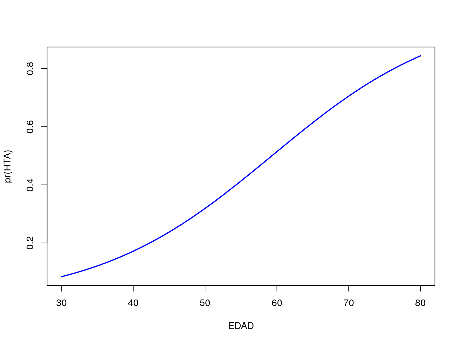

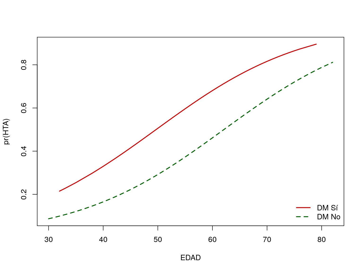
Regresión logística multivariante

• Podemos ahora usar la regresión logística para ajustar el efecto de la edad sobre la HTA según que el sujeto sea o no diabético: \[\pi\left(I_{DM},\textrm{Edad}\right)=\Pr\left(HTA\left|I_{DM},\textrm{Edad}\right.\right)=\] \[\frac{\exp\left(\beta_{0}+\beta_{1}I_{DM}+\beta_{2}\textrm{Edad}\right)}{1+\exp\left(\beta_{0}+\beta_{1}I_{DM}+\beta_{2}\textrm{Edad}\right)}\]

• En este caso: \(\beta_0\) = -4.55068, \(\beta_1\) = 0.90966, \(\beta_2\) = 0.07328

• La OR de HTA con DM ajustada por edad es entonces: \[ e^{\beta_1} = e^{0.90966} = 2.48348 \]

• A la misma edad padecer DM incrementa en 2.48 veces el riesgo de HTA.

mg <- glm(HTA_OMS ~ DM + EDAD, data=telde, family=binomial)
summary(mg)

## 
## Call:
## glm(formula = HTA_OMS ~ DM + EDAD, family = binomial, data = telde)
## 
## Deviance Residuals: 
##     Min       1Q   Median       3Q      Max  
## -2.1255  -0.7804  -0.5432   0.9044   2.2104  
## 
## Coefficients:
##              Estimate Std. Error z value Pr(>|z|)    
## (Intercept) -4.550680   0.348603 -13.054  < 2e-16 ***
## DMSí         0.909660   0.219401   4.146 3.38e-05 ***
## EDAD         0.073285   0.006818  10.748  < 2e-16 ***
## ---
## Signif. codes:  0 '***' 0.001 '**' 0.01 '*' 0.05 '.' 0.1 ' ' 1
## 
## (Dispersion parameter for binomial family taken to be 1)
## 
##     Null deviance: 1282.8  on 1029  degrees of freedom
## Residual deviance: 1081.5  on 1027  degrees of freedom
## AIC: 1087.5
## 
## Number of Fisher Scoring iterations: 4

Odds-Ratio

exp(coef(mg))

## (Intercept)        DMSí        EDAD 
##  0.01056002  2.48347866  1.07603696

exp(confint(mg))

## Waiting for profiling to be done...

##                   2.5 %     97.5 %
## (Intercept) 0.005256831 0.02064005
## DMSí        1.619664315 3.83379057
## EDAD        1.061975094 1.09077065

Representamos gráficamente la relación entre la probabilidad de padecer HTA y la edad según que el sujeto sea o no diabético:

• A todas las edades el riesgo de HTA es mayor entre los que padecen DM.

Regresión logística multivariante

Por último estudiamos la asociación de DM con HTA ajustando simultáneamente por IR y Edad:

\[\pi\left(I_{DM},I_{IR},\textrm{Edad}\right)=\Pr\left(HTA\left|I_{DM},I_{IR},\textrm{Edad}\right.\right)=\]

\[=\frac{\exp\left(\beta_{0}+\beta_{1}I_{DM}+\beta_{2}I_{IR}+\beta_{3}\textrm{Edad}\right)}{1+\exp\left(\beta_{0}+\beta_{1}I_{DM}+\beta_{2}I_{IR}+\beta_{3}\textrm{Edad}\right)}\]

mg2 <- glm(HTA_OMS~DM+IR+EDAD,data=telde,family=binomial)
summary(mg2)

## 
## Call:
## glm(formula = HTA_OMS ~ DM + IR + EDAD, family = binomial, data = telde)
## 
## Deviance Residuals: 
##     Min       1Q   Median       3Q      Max  
## -2.0154  -0.7342  -0.4717   0.8531   2.3655  
## 
## Coefficients:
##              Estimate Std. Error z value Pr(>|z|)    
## (Intercept) -4.965598   0.369248 -13.448  < 2e-16 ***
## DMSí         0.323218   0.236159   1.369    0.171    
## IRSí         1.178958   0.166337   7.088 1.36e-12 ***
## EDAD         0.074358   0.007001  10.621  < 2e-16 ***
## ---
## Signif. codes:  0 '***' 0.001 '**' 0.01 '*' 0.05 '.' 0.1 ' ' 1
## 
## (Dispersion parameter for binomial family taken to be 1)
## 
##     Null deviance: 1282.8  on 1029  degrees of freedom
## Residual deviance: 1031.2  on 1026  degrees of freedom
## AIC: 1039.2
## 
## Number of Fisher Scoring iterations: 4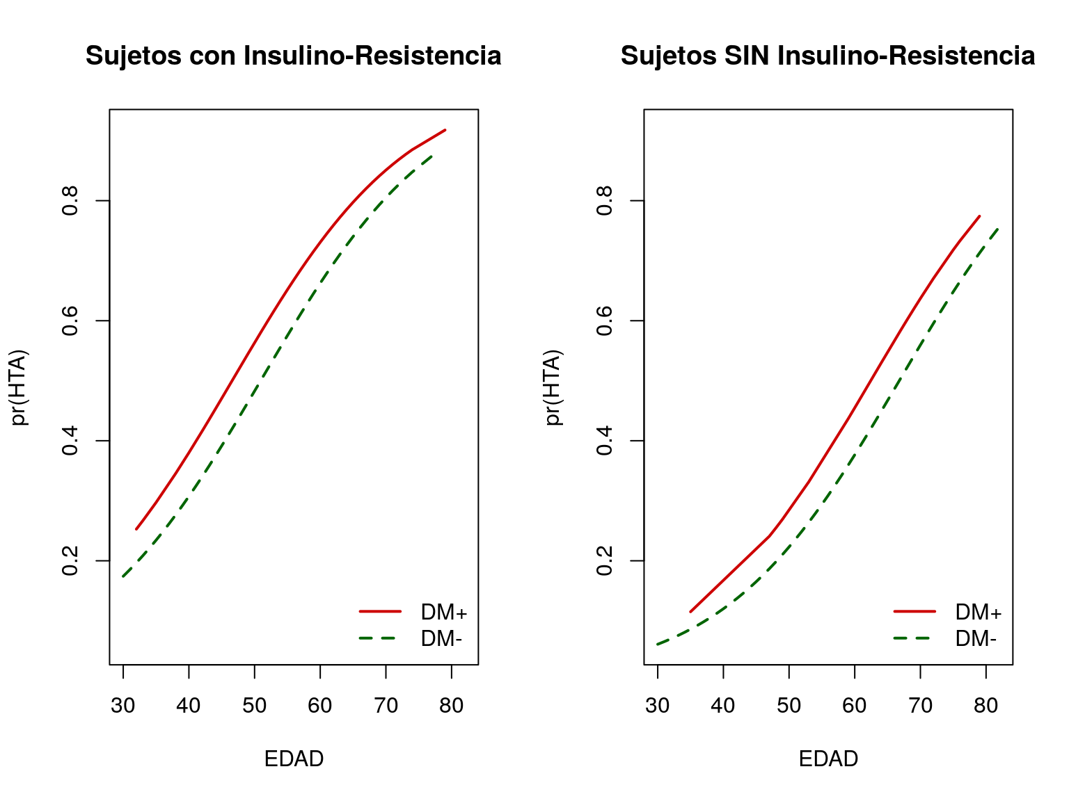

• Si bien en apariencia la probabilidad de HTA a todas las edades es mayor entre los diabéticos, la distancia entre la curva de los DM y los no DM se ha reducido tanto en el grupo de los IR como en el de los no IR. El p-valor 0.171 indica que dicha distancia no es significativa.

Regresión logística multivariante

Resumen de la estimación del modelo: